Where we left off with Part 1 of This Blog we examined the seasonal data as a whole and utilised this data through an ARIMA model to predict the 2018 results. For the calendar year to date, we had an accuracy of 3.88%. While that accuracy is pretty good if you were to use this method to predict inventory requirements you would ideally want even better. The steps described below can be adapted to any seasonal sales forecasting by adjusting the seasonality. As with the last post, we will be utilising Python to conduct our data analysis. The principals however can be utilised in any programming language or even Excel with appropriate extensions installed.
First, let’s try segmenting the data by region to see if each state varies in sales pattern and if running those separately will improve the accuracy of our model.
Let’s look at the patterns of them.
#Import all required libraries
import warnings
import itertools
import numpy as np
import matplotlib.pyplot as plt
import pandas as pd
import statsmodels.api as sm
import matplotlib
from pylab import rcParams
warnings.filterwarnings("ignore")
plt.style.use('fivethirtyeight')

matplotlib.rcParams['axes.labelsize'] = 14
matplotlib.rcParams['xtick.labelsize'] = 12
matplotlib.rcParams['ytick.labelsize'] = 12
matplotlib.rcParams['text.color'] = 'k'
Let’s re-familiarise ourselves with what data we’re dealing with here.
#Import file and print column names
df = pd.read_excel("/NEWMVSALES.xls")
all_cars = pd.DataFrame(df)
print(all_cars.columns)Index(['MEASURE', 'Measure', 'VEHICLE', 'Vehicle Type', 'ASGS_2011', 'Region',
'TSEST', 'Adjustment Type', 'FREQUENCY', 'Frequency', 'TIME', 'Time',
'Value', 'Flag Codes', 'Flags'],
dtype='object')print(all_cars.head())MEASURE Measure VEHICLE Vehicle Type ASGS_2011 Region \
0 1 Number 100 Passenger vehicles 1 New South Wales
1 1 Number 100 Passenger vehicles 1 New South Wales
2 1 Number 100 Passenger vehicles 1 New South Wales
3 1 Number 100 Passenger vehicles 1 New South Wales
4 1 Number 100 Passenger vehicles 1 New South Wales
TSEST Adjustment Type FREQUENCY Frequency TIME Time Value \
0 20 Seasonally Adjusted M Monthly 1994-01 Jan-1994 13107.8
1 20 Seasonally Adjusted M Monthly 1994-02 Feb-1994 13710.6
2 20 Seasonally Adjusted M Monthly 1994-03 Mar-1994 13562.4
3 20 Seasonally Adjusted M Monthly 1994-04 Apr-1994 13786.9
4 20 Seasonally Adjusted M Monthly 1994-05 May-1994 13871.1
Flag Codes Flags
0 NaN NaN
1 NaN NaN
2 NaN NaN
3 NaN NaN
4 NaN NaNNow let’s reduce the columns to only the ones we require.
| Vehicle Type | Region | TIME | Value |
| Passenger vehicles | New South Wales | 1994-01 | 13107.8 |
| Passenger vehicles | New South Wales | 1994-02 | 13710.6 |
| Passenger vehicles | New South Wales | 1994-03 | 13562.4 |
| Passenger vehicles | New South Wales | 1994-04 | 13786.9 |
| Passenger vehicles | New South Wales | 1994-05 | 13871.1 |
Finally, let’s set the index for the TIME values so our data is neatly organised
#convert the 'TIME' column to a datetime values
all_cars['TIME'] = pd.to_datetime(all_cars['TIME'])

#sort the values by date
all_cars.sort_values('TIME')

#index the Values and set index for TIME variable
all_cars['Value'].reset_index()
all_cars = all_cars.set_index('TIME')
all_cars.indexDatetimeIndex(['1994-01-01', '1994-02-01', '1994-03-01', '1994-04-01',
'1994-05-01', '1994-06-01', '1994-07-01', '1994-08-01',
'1994-09-01', '1994-10-01',
...
'2017-03-01', '2017-04-01', '2017-05-01', '2017-06-01',
'2017-07-01', '2017-08-01', '2017-09-01', '2017-10-01',
'2017-11-01', '2017-12-01'],
dtype='datetime64[ns]', name='TIME', length=31104, freq=None)Now that the boring part of the setup is done, let’s graph the data by Region and Vehicle Type to see which one we think is most likely to yield the most accurate results.
In order to do this we’re going to iterate over the Region variables first and graph each one
#Find all values in Region column
locations = all_cars['Region'].unique()

#Save a new dataframe with the Vehicle Type variable locked to 'Total Vehicles'
cars = all_cars.loc[all_cars['Vehicle Type'] == 'Total Vehicles']

#Iterate over all values in the Region column
for l in locations:

#Temporarily lock the location to each Region
car_by_location = cars.loc[cars['Region'] == l]

#Plot each Region's sales values
y = car_by_location['Value']
y.plot(figsize=(20, 15), x = None)
plt.title(l)
plt.show()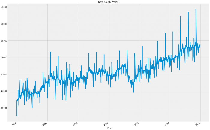
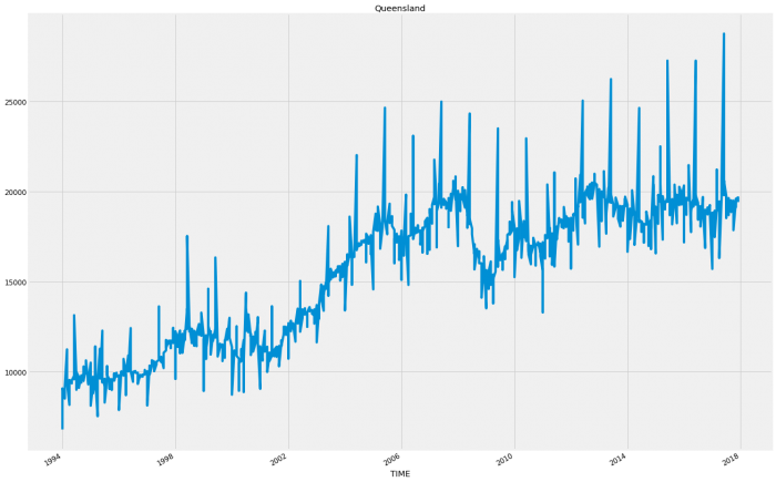
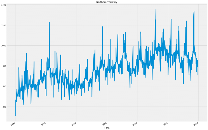
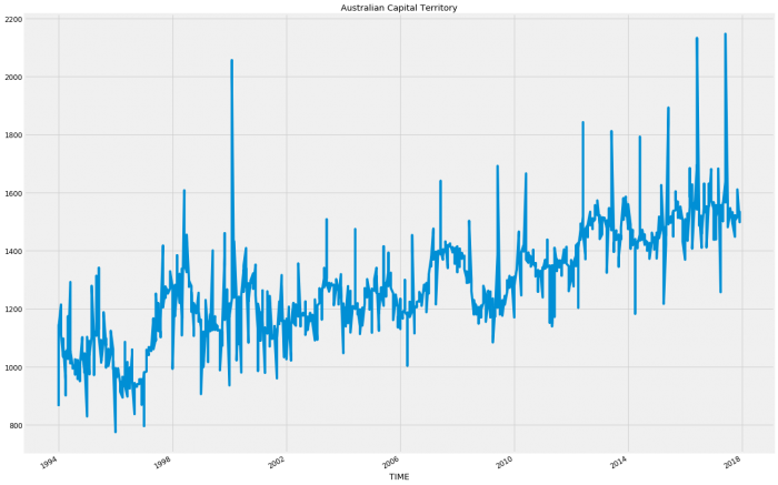
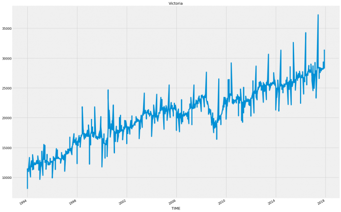
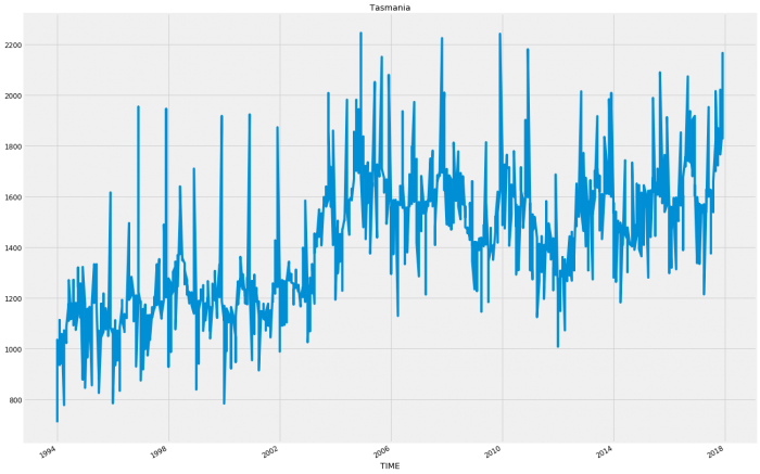
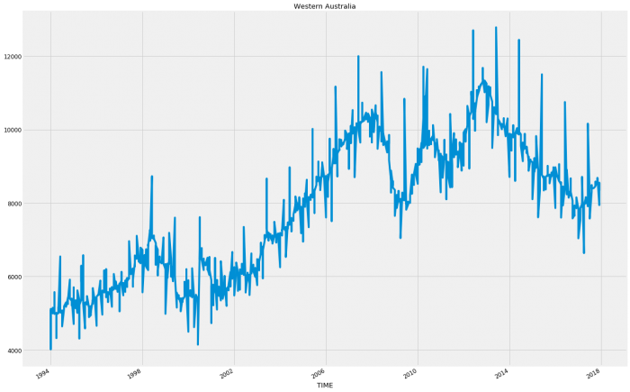
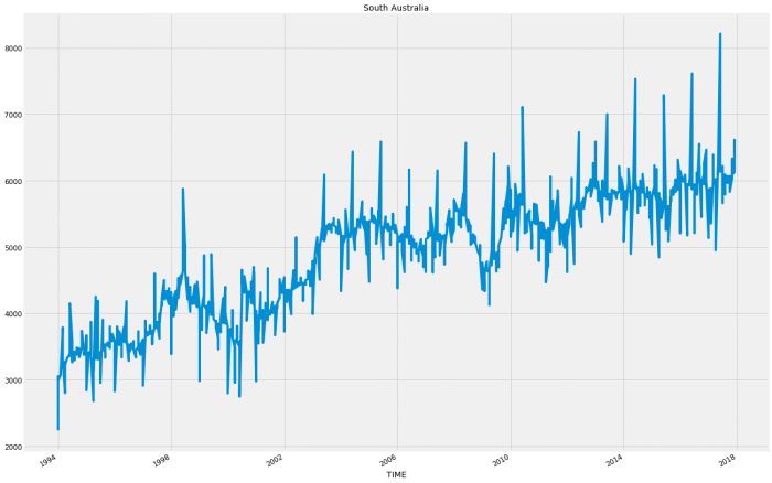
So for the most part each state follows a relatively consistent pattern except Western Australia and Northern Territory which have started to decline in sales. This decline could account for an inaccuracy as these states following a different pattern will be hard to model when wrapped up in with the rest of the results.
Before trialling this theory in a model, let’s have a look at the Vehicle Type data.
#Find all values in Vehicle Type column
car_type = all_cars['Vehicle Type'].unique()

#Save a new dataframe with the Region variable locked to 'Australia'
all_locations = all_cars.loc[all_cars['Region'] == 'Australia']

#Iterate over all values in the Vehicle Type column
for c in car_type:

#Temporarily lock the location to each Vehicle Type
cars_by_type = all_locations.loc[all_locations['Vehicle Type'] == c]

#Plot each Vehicle Type's sales values
y = car_by_type['Value']
y.plot(figsize=(20, 15), x = None)
plt.title(c)
plt.show()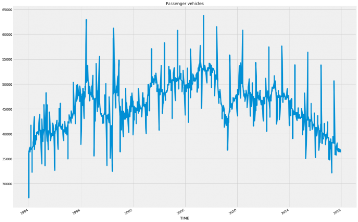
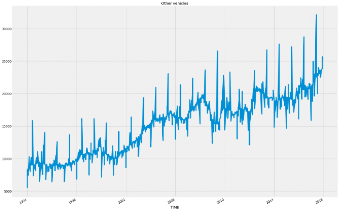
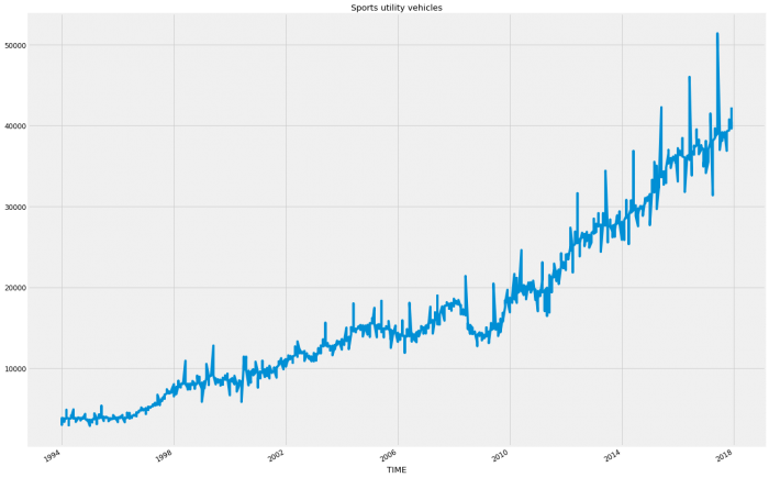
Apparently, the country has gone SUV crazy! I would suspect that like the regional data in Western Australia and Northern Territory; the decline in Passenger Vehicles and the somewhat flattening of Other Vehicles will be skewing the overall pattern so let’s run both. So we’re going to run a modified version of the code from the last blog. We want to do it all in one go this time so that we can iterate through the variables otherwise doing so manually would be immensely time-consuming. Once run, the results will be placed into a column on a new data frame before producing a total column for easier reading later. Finally, we will write the dataframe to a file for future use.
#Trial running iteration over Region segmentation to understand it's effect on accuracy

#Save dictionaries and list for use within the iteration
compiled_df_location = pd.DataFrame()
results_list = []
results_dict = {}

#Create arrays in order to run iteration of all variables
states = np.array(['Northern Territory', 'Queensland', 'New South Wales', 'Australian Capital Territory',
          'Victoria', 'Tasmania', 'South Australia'])

#Set parameters for a progress bar in order to display during processing to give assurance that the program hasn't stalled
pbar = tqdm(total = len(states))
pbar.set_description("Processing")

#Iterate over all regions
for l in states:

    #Create temporary dataframe from the original at the start using the current variables
    car_iter = df.loc[(df['Adjustment Type'] == 'Original') & (df['Vehicle Type'] == 'Total Vehicles') & (df['Region'] == l)]

    #Index and sort values by time
    car_iter['TIME'] = pd.to_datetime(car_iter['TIME'])
    car_iter.sort_values('TIME')
    car_iter['Value'].reset_index()
    car_iter = car_iter.set_index('TIME')
    car_iter.index

    #Create series with sales volume to run through the model
    y = car_iter['Value']

    #Run test SARIMAX model
    p = d = q = range(0, 2)
    pdq = list(itertools.product(p, d, q))
    seasonal_pdq = [(x[0], x[1], x[2], 12) for x in list(itertools.product(p, d, q))]
    for param in pdq:
        for param_seasonal in seasonal_pdq:
            try:
                mod = sm.tsa.statespace.SARIMAX(y,
                                            order=param,
                                            seasonal_order=param_seasonal,
                                            enforce_stationarity=False,
                                            enforce_invertibility=False)
                results = mod.fit()
                #Save results into a list for the purpose of finding the minimum result
                results_list.append(results.aic)
                #Save parameters to be able to find corresponding parmeters to the minimum result
                x = [param, param_seasonal]
                results_dict[results.aic] = x
            except:
                continue

    #Save appropriate parameters for use in the actual model
    rl = min(results_list)
    p1 = results_dict[rl][0]
    p2 = results_dict[rl][1]

    #Run model
    mod = sm.tsa.statespace.SARIMAX(y,
                                order=p1,
                                seasonal_order=p2,
                                enforce_stationarity=False,
                                enforce_invertibility=False)
    results = mod.fit()
    pred_uc = results.get_forecast(steps = 48)
    pred_ci = pred_uc.conf_int()

    #Save results to dataframe
    prediction_4_year = pd.DataFrame(pred_uc.predicted_mean)

    #Create column names and apply to the top of the dataframe
    column_2 = l
    compiled_df_location[column_2] = prediction_4_year[0]

    pbar.update(1)

#Create totals column and append to the end of the dataframe
compiled_df_location.index.name = 'TIME'
compiled_df_location['Total'] = compiled_df_location.iloc[:,-21:].sum(axis = 1)

#Write dataframe to csv
compiled_df_location.to_csv("/4_year_forecast_all_regions_total_vehicles.xls")
print("file written")
Now let’s look at the results
FYTD = compiled_df_location['Total'].loc['2018-01-01':'2018-10-01']
FYTD.loc['TOTAL'] = FYTD.sum()

actuals_total = 971723
variance = FYTD['TOTAL'] - actuals_total
variance_percentage = round(((FYTD['TOTAL'] / actuals_total - 1) * 100), 2)

print('total prediction YTD for 2018 was %.0f' % (FYTD['TOTAL']))
print('total actuals YTD for 2018 was %.0f' % (actuals_total))
print('total variance is %0.0f or %0.2f%%' % (variance, variance_percentage,))
total prediction YTD for 2018 was 927321
total actuals YTD for 2018 was 971723
total variance is -44402 or -4.57%In Part 1 of This Blog, the results were 3.88% so we haven’t improved on those results yet. Let’s try running the vehicle types and see if that will make a difference
#Trial running iteration over Vehicle Types segmentation to understand it's effect on accuracy

#Save dictionaries and list for use within the iteration
compiled_df_vehicle = pd.DataFrame()
results_list = []
results_dict = {}

#Create arrays in order to run iteration of all variables
vehicle_types = np.array(['Other vehicles', 'Passenger vehicles', 'Sports utility vehicles'])

#Set parameters for a progress bar in order to display during processing to give assurance that the program hasn't stalled
pbar = tqdm(total = len(vehicle_types))
pbar.set_description("Processing")

#Iterate over all vehicle types
for v in vehicle_types:

    #Create temporary dataframe from the original at the start using the current variables
    car_iter = df.loc[(df['Adjustment Type'] == 'Original')  & (df['Vehicle Type'] == v) & (df['Region'] == 'Australia')]

    #Index and sort values by time
    car_iter['TIME'] = pd.to_datetime(car_iter['TIME'])
    car_iter.sort_values('TIME')
    car_iter['Value'].reset_index()
    car_iter = car_iter.set_index('TIME')
    car_iter.index

    #Create series with sales volume to run through the model
    y = car_iter['Value']

    #Run test SARIMAX model
    p = d = q = range(0, 2)
    pdq = list(itertools.product(p, d, q))
    seasonal_pdq = [(x[0], x[1], x[2], 12) for x in list(itertools.product(p, d, q))]
    for param in pdq:
        for param_seasonal in seasonal_pdq:
            try:
                mod = sm.tsa.statespace.SARIMAX(y,
                                            order=param,
                                            seasonal_order=param_seasonal,
                                            enforce_stationarity=False,
                                            enforce_invertibility=False)
                results = mod.fit()
                #Save results into a list for the purpose of finding the minimum result
                results_list.append(results.aic)
                #Save parameters to be able to find corresponding parmeters to the minimum result
                x = [param, param_seasonal]
                results_dict[results.aic] = x
            except:
                continue

    #Save appropriate parameters for use in the actual model
    rl = min(results_list)
    p1 = results_dict[rl][0]
    p2 = results_dict[rl][1]

    #Run model
    mod = sm.tsa.statespace.SARIMAX(y,
                                order=p1,
                                seasonal_order=p2,
                                enforce_stationarity=False,
                                enforce_invertibility=False)
    results = mod.fit()
    pred_uc = results.get_forecast(steps = 48)
    pred_ci = pred_uc.conf_int()

    #Save results to dataframe
    prediction_4_year = pd.DataFrame(pred_uc.predicted_mean)

    #Create column names and apply to the top of the dataframe
    column_2 = v
    compiled_df_vehicle[column_2] = prediction_4_year[0]

    pbar.update(1)

#Create totals column and append to the end of the dataframe
compiled_df_vehicle.index.name = 'TIME'
compiled_df_vehicle['Total'] = compiled_df_vehicle.iloc[:,-21:].sum(axis = 1)

#Write dataframe to csv
compiled_df_vehicle.to_csv("/4_year_forecast_all_vehicle_types_Australia.xls")
print("file written")
FYTD = compiled_df_location['Total'].loc['2018-01-01':'2018-10-01']
FYTD.loc['TOTAL'] = FYTD.sum()

actuals_total = 971723
variance = FYTD['TOTAL'] - actuals_total
variance_percentage = round(((FYTD['TOTAL'] / actuals_total - 1) * 100), 2)

print('total prediction YTD for 2018 was %.0f' % (FYTD['TOTAL']))
print('total actuals YTD for 2018 was %.0f' % (actuals_total))
print('total variance is %0.0f or %0.2f%%' % (variance, variance_percentage,))
total prediction YTD for 2018 was 1010168
total actuals YTD for 2018 was 971723
total variance is 38445 or 3.96%Ok, so that’s close to the previous results and may come in handy if you were looking at inventory ordering because at least you would have a better idea of what to order. But the goal was to improve on overall accuracy so let’s see what else we can do. We’re going to try iterating over both variables, so for each region, we’re going to run through each vehicle type. This will produce 21 segments so let’s see if this improves accuracy.
#Trial running iteration over both Region and Vehicle Type segmentation to understand it's effect on accuracy

#Save dictionaries and list for use within the iteration
compiled_df_all = pd.DataFrame()
results_list = []
results_dict = {}

#Create arrays in order to run iteration of all variables
states = np.array(['Northern Territory', 'Queensland', 'New South Wales', 'Australian Capital Territory',
          'Victoria', 'Tasmania', 'South Australia'])
vehicle_types = np.array(['Other vehicles', 'Passenger vehicles', 'Sports utility vehicles'])

#Set parameters for a progress bar in order to display during processing to give assurance that the program hasn't stalled
pbar = tqdm(total = len(states) * len(vehicle_types))
pbar.set_description("Processing")

#Iterate over all regions
for l in states:
    #Iterate over all vehicle types
    for v in vehicle_types:

        #Create temporary dataframe from the original at the start using the current variables
        car_iter = df.loc[(df['Adjustment Type'] == 'Original') & (df['Vehicle Type'] == v) & (df['Region'] == l)]

        #Index and sort values by time
        car_iter['TIME'] = pd.to_datetime(car_iter['TIME'])
        car_iter.sort_values('TIME')
        car_iter['Value'].reset_index()
        car_iter = car_iter.set_index('TIME')
        car_iter.index

        #Create series with sales volume to run through the model
        y = car_iter['Value']

        #Run test SARIMAX model
        p = d = q = range(0, 2)
        pdq = list(itertools.product(p, d, q))
        seasonal_pdq = [(x[0], x[1], x[2], 12) for x in list(itertools.product(p, d, q))]
        for param in pdq:
            for param_seasonal in seasonal_pdq:
                try:
                    mod = sm.tsa.statespace.SARIMAX(y,
                                                order=param,
                                                seasonal_order=param_seasonal,
                                                enforce_stationarity=False,
                                                enforce_invertibility=False)
                    results = mod.fit()
                    #Save results into a list for the purpose of finding the minimum result
                    results_list.append(results.aic)
                    #Save parameters to be able to find corresponding parmeters to the minimum result
                    x = [param, param_seasonal]
                    results_dict[results.aic] = x
                except:
                    continue

        #Save appropriate parameters for use in the actual model
        rl = min(results_list)
        p1 = results_dict[rl][0]
        p2 = results_dict[rl][1]

        #Run model
        mod = sm.tsa.statespace.SARIMAX(y,
                                    order=p1,
                                    seasonal_order=p2,
                                    enforce_stationarity=False,
                                    enforce_invertibility=False)
        results = mod.fit()
        pred_uc = results.get_forecast(steps = 48)
        pred_ci = pred_uc.conf_int()

        #Save results to dataframe
        prediction_4_year = pd.DataFrame(pred_uc.predicted_mean)

        #Create column names and apply to the top of the dataframe
        column_2 = v + " & " + l
        compiled_df_all[column_2] = prediction_4_year[0]

        pbar.update(1)

#Create totals column and append to the end of the dataframe
compiled_df_all.index.name = 'TIME'
compiled_df_all['Total'] = compiled_df_all.iloc[:,-21:].sum(axis = 1)

#Write dataframe to csv
compiled_df_all.to_csv("/4_year_forecast_all_region_and_vehicle_types.xls")
print("file written")
FYTD = compiled_df_all['Total'].loc['2018-01-01':'2018-10-01']
FYTD.loc['TOTAL'] = FYTD.sum()

actuals_total = 971723
variance = FYTD['TOTAL'] - actuals_total
variance_percentage = round(((FYTD['TOTAL'] / actuals_total - 1) * 100), 2)

print('total prediction YTD for 2018 was %.0f' % (FYTD['TOTAL']))
print('total actuals YTD for 2018 was %.0f' % (actuals_total))
print('total variance is %0.0f or %0.2f%%' % (variance, variance_percentage,))
total prediction YTD for 2018 was 932181
total actuals YTD for 2018 was 971723
total variance is -39542 or -4.07%Still not what we wanted, sometimes over-segmentation can do this. If we had access to the detailed reports for 2018 it would be very worthwhile graphing these results against the actual results. This would help to see if there is an anomaly causing this and we could perhaps manually improve this.
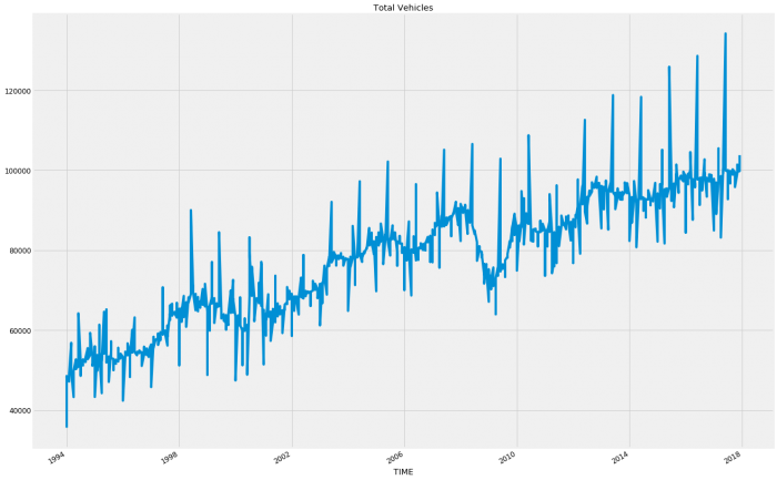
In the graphs, we observed previously that there was a fall in sales during the Global Financial Crisis that changed the pattern for nearly 2 years. The pattern returned to be relatively normal in 2010 so as our final model we will only run the years 2010 to 2017 to see if removing this anomaly will improve the results.
#Trial running for results 2010-2017 to understand it's effect on accuracy
#For sakes of reusing previous code we will simply replace the parameters for states and vehicle_typles with the totals
#This will of course only be one iteration and could be redone for faster processing
#However i have left it as is to demonstrate the versitility of such a code

#Save dictionaries and list for use within the iteration
compiled_df = pd.DataFrame()
results_list = []
results_dict = {}

#Create arrays in order to run iteration of all variables
states = np.array(['Australia'])
vehicle_types = np.array(['Total Vehicles'])

#Set parameters for a progress bar in order to display during processing to give assurance that the program hasn't stalled
pbar = tqdm(total = len(states) * len(vehicle_types))
pbar.set_description("Processing")

#Iterate over all regions
for l in states:
    #Iterate over all vehicle types
    for v in vehicle_types:

        #Create temporary dataframe from the original at the start using the current variables
        car_iter = df.loc[(df['Adjustment Type'] == 'Original') & (df['Vehicle Type'] == v) & (df['Region'] == l)]

        #Index and sort values by time
        car_iter['TIME'] = pd.to_datetime(car_iter['TIME'])
        car_iter.sort_values('TIME')
        car_iter['Value'].reset_index()
        car_iter = car_iter.set_index('TIME')
        car_iter.index
        car_iter = car_iter.loc['2010-01-01':]

        #Create series with sales volume to run through the model
        y = car_iter['Value']

        #Run test SARIMAX model
        p = d = q = range(0, 2)
        pdq = list(itertools.product(p, d, q))
        seasonal_pdq = [(x[0], x[1], x[2], 12) for x in list(itertools.product(p, d, q))]
        for param in pdq:
            for param_seasonal in seasonal_pdq:
                try:
                    mod = sm.tsa.statespace.SARIMAX(y,
                                                order=param,
                                                seasonal_order=param_seasonal,
                                                enforce_stationarity=False,
                                                enforce_invertibility=False)
                    results = mod.fit()
                    #Save results into a list for the purpose of finding the minimum result
                    results_list.append(results.aic)
                    #Save parameters to be able to find corresponding parmeters to the minimum result
                    x = [param, param_seasonal]
                    results_dict[results.aic] = x
                except:
                    continue

        #Save appropriate parameters for use in the actual model
        rl = min(results_list)
        p1 = results_dict[rl][0]
        p2 = results_dict[rl][1]

        #Run model
        mod = sm.tsa.statespace.SARIMAX(y,
                                    order=p1,
                                    seasonal_order=p2,
                                    enforce_stationarity=False,
                                    enforce_invertibility=False)
        results = mod.fit()
        pred_uc = results.get_forecast(steps = 48)
        pred_ci = pred_uc.conf_int()

        #Save results to dataframe
        prediction_4_year = pd.DataFrame(pred_uc.predicted_mean)

        #Create column names and apply to the top of the dataframe
        column_2 = v + " & " + l
        compiled_df[column_2] = prediction_4_year[0]

        pbar.update(1)

#Create totals column and append to the end of the dataframe
compiled_df.index.name = 'TIME'
compiled_df['Total'] = compiled_df.iloc[:,-21:].sum(axis = 1)

#Write dataframe to csv
compiled_df.to_csv("/4_year_forecast_total_2010-2017.xls")
print("file written")
FYTD = compiled_df['Total'].loc['2018-01-01':'2018-10-01']
FYTD.loc['TOTAL'] = FYTD.sum()

actuals_total = 971723
variance = FYTD['TOTAL'] - actuals_total
variance_percentage = round(((FYTD['TOTAL'] / actuals_total - 1) * 100), 2)

print('total prediction YTD for 2018 was %.0f' % (FYTD['TOTAL']))
print('total actuals YTD for 2018 was %.0f' % (actuals_total))
print('total variance is %0.0f or %0.2f%%' % (variance, variance_percentage,))
total prediction YTD for 2018 was 1006149
total actuals YTD for 2018 was 971723
total variance is 34426 or 3.54%Excellent! We’ve improved on the original model. Once again if this was a real-world scenario we could run this shorter time period across the other models. Alternatively, we could remove them so that we were running both before and after because in general the more clean data that a model has to work with, the more accurate the results. Perhaps a different post utilising a different model.
If you are interested in the source code for this blog see my GitHub.
Leave a Reply